Learn you Galois Fields for Great Good (04)
Navigation | table of contents | previous | next
Polynomial Arithmetic
This is part 4 of a series on Abstract Algebra. In this part, we'll give a refresher on polynomial arithmetic: addition, subtraction, multiplication, and division. The fact that we can define these four operations over polynomials should give you a very big hint about where we are going. 😉
Polynomials
An nth-order polynomial is any expression of the form where c_n != 0:
c_n * x^n + c_{n-1} * x^(n-1) + ... + c_2 * x^2 + c_1 * x + c_0
In particular, these are all 4th-order polynomials:
2x^4 + x^3 + 10x + 7
x^4 + 3x^2 + 4x
3x^4 + 1
x^4
These are not 4th-order polynomials:
x^3              [3rd-order]
2x^2 + 1         [2nd-order]
3x^5 + x^4       [5th-order]
Polynomial Arithmetic
Our goal is to add, subtract, multiply and divide polynomials. To be clear, we aren't doing these operations over normal
numbers but the polynomials themselves. We don't care about one particular x=k. We care about all x's. The polynomial itself
is the "weird number".
In other words, we want to add/multiply the entire graph of points.
Consider these:
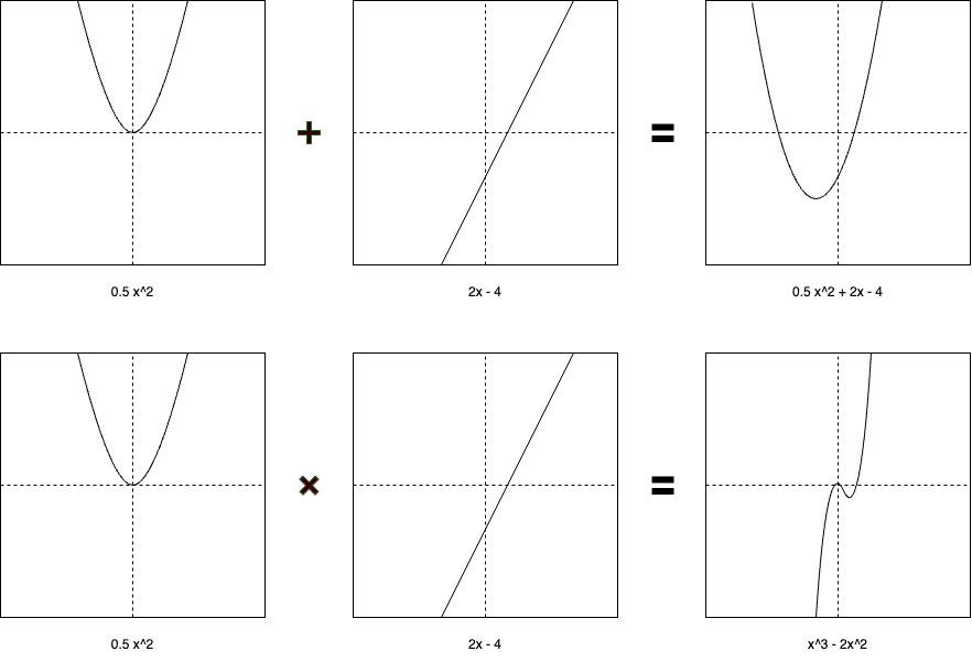
Hopefully that helps!
Addition and Subtraction
Adding polynomials is straight-forward. Just group like-terms and add the coefficients:
(2x^3 + 3) + (x^3 + 3x^2 + 6)
(2x^3 + x^3) + (3x^2 + 0x^2) + (3 + 6)
3x^3 + 3x^2 + 9
It's also easy to negate a polynomial:
-(x^3 + 3x^2 + 6) = -x^3 - 3x^2 - 6
So, we have subtraction easily:
(2x^3 + 3) - (x^3 + 3x^2 + 6)
(2x^3 + 3) + -(x^3 + 3x^2 + 6)
(2x^3 + 3) + (-x^3 - 3x^2 - 6)
(2x^3 - x^3) + (3x^2 - 0x^2) + (3 - 6)
(2 - 1)x^3 + (3 - 0)x^2 + (3 - 6)
x^3 + 3x^2 - 3
Naturally a negation is an additive-inverse:
x^3 + 3x^2 + 6 + -(x^3 + 3x^2 + 6)
(1 - 1)x^3 + (3 - 3)x^2 + (6 - 6)
(0)x^3 + (0)x^2 + (0)
0
Generalizing, for addition we can simply add coefficients. For the polynomials A, B
with coefficients a_i and b_i:
A = a_n * x^n + a_{n-1} * x^(n-1) + ... + a_2 * x^2 + a_1 * x + a_0
B = b_n * x^n + b_{n-1} * x^(n-1) + ... + b_2 * x^2 + b_1 * x + b_0
The polynomial C = A + B has coefficients c_i = (a_i + b_i):
C = A + B = (a_n + b_n) * x^n + (a_{n-1} + b_{n-1}) * x^(n-1) + ... + (a_2 + b_2) * x^2 + (a_1 + b_2) * x + (a_0 + b_0)
C = A + B = c_n * x^n + c_{n-1} * x^(n-1) + ... + c_2 * x^2 + c_1 * x + c_0
Exercise: Compute (x^4 + 1) + (3x^4 + x^2)
Exercise: Compute (5) + (x^2 - 4)
Exercise: Compute (-x^2 + 3) - (-x^2 + 3)
Vector Notation
Since working with polynomials in the standard notation is verbose and tedious, we'll occasionally adopt various alternative notations or representations. Often if you read about some application of Galois Fields, the author will assume you are familiar with these alternative representations and will switch between them intuitively. This can be a big source of confusion. Let's clear it up by being explicit.
Here we introduce Vector Notation.
Instead of writing the verbose polynomial:
x^3 + 3x^2 + 6
We will write a row-vector containing only the coefficients:
[1, 3, 0, 6]
We can see that this is a valid representation by performing a dot-product with the monomial basis vector:
[1, 3, 0, 6] dot [x^3, x^2, x, 1] = x^3 + 3x^2 + 6
With this representation, our first addition above becomes a simple vector addition:
[2, 0, 0, 3] + [1, 3, 0, 6]
[3, 3, 0, 9]
Much better!
Exercise: Convert x^4 + 1 to vector notation
Exercise: Convert 3x^4 + x^2 to vector notation
Exercise: Sum the previous two answers (vectors) and convert to polynomial representation. This should be the same as your answer to
(x^4 + 1) + (3x^4 + x^2)
Multiplication
We now want to multiply polynomials. Let's start with a simple two-term binomial multiply:
(2x + 3) * (3x + 1)
(2x * 3x) + (2x * 1) + (3 * 3x) + (3 * 1)
6x^2 + 2x + 9x + 3
6x^2 + (2+9)x + 3
6x^2 + 11x + 3
Here for the binomial case, we can just use the familiar FOIL method. But for larger order polynomials, it gets more complicated:
(2x^2 + x + 3) * (3x^2 + 4x + 1)
(2x^2 * 3x^2) + (2x^2 * 4x) + (2x^2 * 1) + (x * 3x^2) + (x * 4x) + (x * 1) + (3 * 3x^2) + (3 * 4x) + (3 * 1)
6x^4 + 8x^3 + 2x^2 + 3x^3 + 4x^2 + x + 9x^2 + 12x + 3
6x^4 + 11x^3 + 15x^2 + 13x + 3
Consider a 5th order polynomial. There are 6 different multiplications that will produce an x^5 term:
1   * x^5 = x^5
x   * x^4 = x^5
x^2 * x^3 = x^5
x^3 * x^2 = x^5
x^4 * x   = x^5
x^5 * 1   = x^5
This gets worse as the order increases. Notice that a 100th-order polynomial will have 101 terms contributing
to it's resulting x^100 term!
Further, notice that the order of the polynomial increases as a result of a multiplication.
From our simple example above:
(1st order) * (1st order) = (2nd order)
And for the 5th order, we'd have one term where ax^5 * bx^5 = (a*b)x^10, so:
(5th order) * (5th order) = (10th order)
A 100th-order polynomial multiplied by another 100th-order polynomial will result in a 200th-other polynomial!
Exercise: Compute (x^4 + 2x) * (3x^2 + x + 4). What is the order of the result? How many terms contribute to
the resulting x^2 term?
Multiplication is a Convolution
Hopefully, its clear now that multiplication is not a simple sum of coefficients. Instead its a sum of many smaller multiplications. This operation appears in enough contexts in mathematics that it has a well-known name: A Convolution.
We are doing the following:
(2x + 3) * (3x + 1)
[2, 3] * [3, 1]                        [change to vector notation]
convolve([2, 3], [3, 1])               [multiplication is a convolution]
[6, 11, 3]                             [compute the convolution of two row vectors]
6x^2 + 11x + 3                         [change back to polynomial notation]
Exercise: Check the multiplication above using the ordinary term-by-term, non-convolution approach.
In interest of time, I'm not going to dig deeper into the convolution in this post. However, it's important to recognize this structure for further optimizations. In particular, the convolution can be transformed into a simpler problem (that does behave more like combining like terms) by using a Fast Fourier Transform (FFT). We may cover this in a future article.
Luckily, if your goal is to just understand and use Galois Fields, this can just be viewed as an implementation optimization. One doesn't need to understand the connection to Convolution and FFT in order to appreciate and utilize these Fields.
But, if you're a curious cat, a well-known math YouTuber made a nice video on the subject (here). Highly recommended 👍
Division
We've already seen one case where division works. We can just reframe our multiplication above:
(6x^2 + 11x + 3) / (2x + 3) = (3x + 1)
However, not all division will work, consider:
(2x + 4) / (2x + 3) = 1 + ?
This is analogous to normal integer division having remainders:
7 / 2 = 3 remainder 2 [NOTE: 3*2 + 2 = 7]
So we do the same with polynomials:
(2x + 4) / (2x + 3) = 1 remainder 1 [NOTE: 1 * (2x + 3) + 1 = 2x + 4]
This is known as long-division of polynomials. It works exactly like long-division of the natural numbers, it's just more verbose:
                    2x^3 + -3x^2 + 6.5x - 15.5  R 60
          -----------------------------------------
(2x + 4) |   4x^4 + 2x^3 + x^2 + -5x - 2
           -(4x^4 + 8x^3)
             -----------
                   -6x^3 +  x^2 + -5x - 2
                 -(-6x^3 -12x^2)
                   ------------
                          13x^2 + -5x - 2
                        -(13x^2 + 26x)
                          -----------
                                 -31x - 2
                               -(-31x - 62)
                                 ---------
                                        60 (remainder)
Checking:
(2x + 4) * (2x^3 + -3x^2 + 6.5x - 15.5) + 60
(4x^4) + (8x^3 + -6x^3) + (-12x^2 + 13x^2) + (26x - 31x) + (-62) + 60
4x^4 + 2x^3 + x^2 + -5x - 2
Long-division of polynomials is tedious, verbose, and error-prone. You don't have to be an expert at it, but you should be familiar enough to know that division of polynomials isn't magic. It's just rote calculation.
Here are some additional resources to help you attain mastery:
Multiplicative-inverses
When we introduced the concept of a field, we observed that addition and multiplication were the only two operators we needed to consider given that we had access to additive-inverses and multiplicative-inverses.
We established above that additive-inverses are straightforward, but what about multiplicative-inverses? Sadly no.
Suppose we wanted the inverse of A = 2x + 1:
A * inv(A) = 1
(2x + 1) * inv(A) = 1
inv(A) = 1 / (2x + 1)
inv(A) = 0 rem 1
Uh oh!
The only polynomial that works is 1 since 1/1 = 1. This is a big problem and it means that our polynomials are NOT a Field! Disaster, right?
It turns out we can patch this up in the same sort of way we made modular arithmetic work with integers. But that's for next time.